📄 THEORY 📄 Studying the fundamental topics that are Algorithms and Datastructures

Algorithms-and-Datastructures

|| MD Written and Styled in StackEdit.io

INDEX

1. Algorithms
2. Time Complexity
3. Asymptotic notation
4. (to be continued..) Arrays
5. Stacks
6. Stack Applications
7. Recursion
8. Queues
9. Searching
10. Sorting
11. Quick sort
12. Heap sort
13. Trees

Introduction to Data Structures

• Data Structure can be defined as the group of data elements which provides an efficient way of storing and organizing data in the computer so that it can be used efficiently.
• Some examples of Data Structures are arrays, Linked List, Stack, Queue, etc.
• Data Structures are widely used in almost every aspect of Computer Science i.e. Operating System, Compiler Design, Artificial intelligence, Graphics and many more.
• Reference: https://www.javatpoint.com/data-structure-introduction

Basic Terminology

Data structures are the building blocks of any program or the software.

• Choosing the appropriate data structure for a program is the most difficult task for a programmer.

• Following terminology is used as far as data structures are concerned.

• Data: Data can be defined as an elementary value or the collection of values, for example, student's name and its id are the data about the student.

• Group Items: Data items which have subordinate data items are called Group item, for example, name of a student can have first name and the last name.

• Record: Record can be defined as the collection of various data items, for example, if we talk about the student entity, then its name, address, course and marks can be grouped together to form the record for the student.

• File: A File is a collection of various records of one type of entity, for example, if there are 60 employees in the class, then there will be 60 records in the related file where each record contains the data about each employee.

• Attribute and Entity: An entity represents the class of certain objects. it contains various attributes. Each attribute represents the particular property of that entity.

• Field: Field is a single elementary unit of information representing the attribute of an entity.

Need of Data Structures

As applications are getting complexed and amount of data is increasing day by day, there may arise the following problems: Processor speed: To handle very large amount of data, high speed processing is required, but as the data is growing day by day to the billions of files per entity, processor may fail to deal with that much amount of data. Data Search: Consider an inventory size of 106 items in a store, If our application needs to search for a particular item, it needs to traverse 106 items every time, results in slowing down the search process. Multiple requests: If thousands of users are searching the data simultaneously on a web server, then there are the chances that a very large server can be failed during that process In order to solve the above problems, data structures are used. Data is organised to form a data structure in such a way that all items are not required to be searched and required data can be searched instantly.

Advantages of Data Structures

• Efficiency: Efficiency of a program depends upon the choice of data structures.
  • For example: suppose, we have some data and we need to perform the search for a particular record. In that case, if we organize our data in an array, we will have to search sequentially element by element. hence, using array may not be very efficient here. There are better data structures which can make the search process efficient like ordered array, binary search tree or hash tables.
• Reusability: Data structures are reusable, i.e. once we have implemented a particular data structure, we can use it at any other place. Implementation of data structures can be compiled into libraries which can be used by different clients.
• Abstraction: Data structure is specified by the ADT which provides a level of abstraction. The client program uses the data structure through interface only, without getting into the implementation details.
  • Abstract Data type (ADT) is a type (or class) for objects whose behaviour is defined by a set of value and a set of operations. The definition of ADT only mentions what operations are to be performed but not how these operations will be implemented. It does not specify how data will be organized in memory and what algorithms will be used for implementing the operations. It is called “abstract” because it gives an implementation-independent view. The process of providing only the essentials and hiding the details is known as abstraction.

Data Structure Classification

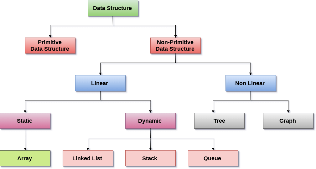
There are two types of data structure available for the programming purpose:

• Primitive data structure

• Non-primitive data structure

• Primitive data structure is a fundamental type of data structure that stores the data of only one type whereas the non-primitive data structure is a type of data structure which is a user-defined that stores the data of different types in a single entity.

• In the case of primitive data structure, it contains fundamental data types such as integer, float, character, pointer, and these fundamental data types can hold a single type of value.

• For example, integer variable can hold integer type of value, float variable can hold floating type of value, character variable can hold character type of value whereas the pointer variable can hold pointer type of value.

• In the case of non-primitive data structure, it is categorized into two parts such as linear data structure and non-linear data structure.

• Linear data structure is a sequential type of data structure, and here sequential means that all the elements in the memory are stored in a sequential manner; for example, element stored after the second element would be the third element, the element stored after the third element would be the fourth element and so on.

• We have different linear data structures holding the sequential values such as Array, Linked list, Stack, Queue. Non-linear data structure is a kind of random type of data structure. The non-linear data structures are Tree and Graph.

• Linear Data Structures: A data structure is called linear if all of its elements are arranged in the linear order. In linear data structures, the elements are stored in non-hierarchical way where each element has the successors and predecessors except the first and last element.

• Types of Linear Data Structures are given below: Arrays: An array is a collection of similar type of data items and each data item is called an element of the array. The data type of the element may be any valid data type like char, int, float or double.

• The elements of array share the same variable name but each one carries a different index number known as subscript. The array can be one dimensional, two dimensional or multidimensional.

• The individual elements of the array age are: age[0], age[1], age[2], age[3],......... age[98], age[99].

• Linked List: Linked list is a linear data structure which is used to maintain a list in the memory. It can be seen as the collection of nodes stored at non-contiguous memory locations. Each node of the list contains a pointer to its adjacent node.

• Stack: Stack is a linear list in which insertion and deletions are allowed only at one end, called top. A stack is an abstract data type (ADT), can be implemented in most of the programming languages. It is named as stack because it behaves like a real-world stack, for example: - piles of plates or deck of cards etc.

• Queue: Queue is a linear list in which elements can be inserted only at one end called rear and deleted only at the other end called front. It is an abstract data structure, similar to stack. Queue is opened at both end therefore it follows First-In-First-Out (FIFO) methodology for storing the data items.

• Non Linear Data Structures: This data structure does not form a sequence i.e. each item or element is connected with two or more other items in a non-linear arrangement. The data elements are not arranged in sequential structure.

• Types of Non Linear Data Structures are given below:

  • Trees:
    • Trees are multilevel data structures with a hierarchical relationship among its elements known as nodes. The bottommost nodes in the hierarchy are called leaf node while the topmost node is called root node. Each node contains pointers to point adjacent nodes. Tree data structure is based on the parent-child relationship among the nodes. Each node in the tree can have more than one children except the leaf nodes whereas each node can have atmost one parent except the root node. Trees can be classified into many categories which will be discussed later in this course.
  • Graphs:
    • Graphs can be defined as the pictorial representation of the set of elements (represented by vertices) connected by the links known as edges. A graph is different from tree in the sense that a graph can have cycle while the tree can not have the one.

Operations on data structure

1. Traversing: Every data structure contains the set of data elements. Traversing the data structure means visiting each element of the data structure in order to perform some specific operation like searching or sorting. Example: If we need to calculate the average of the marks obtained by a student in 6 different subject, we need to traverse the complete array of marks and calculate the total sum, then we will divide that sum by the number of subjects i.e. 6, in order to find the average.

2. Insertion: Insertion can be defined as the process of adding the elements to the data structure at any location. If the size of data structure is n then we can only insert n-1 data elements into it.

3. Deletion: The process of removing an element from the data structure is called Deletion. We can delete an element from the data structure at any random location. If we try to delete an element from an empty data structure then underflow occurs.

4. Searching: The process of finding the location of an element within the data structure is called Searching. There are two algorithms to perform searching, Linear Search and Binary Search. We will discuss each one of them later in this tutorial.

5. Sorting: The process of arranging the data structure in a specific order is known as Sorting. There are many algorithms that can be used to perform sorting, for example, insertion sort, selection sort, bubble sort, etc.

6. Merging: When two lists List A and List B of size M and N respectively, of similar type of elements, clubbed or joined to produce the third list, List C of size (M+N), then this process is called merging

What is an Algorithm?

• What are algorithms?

• Why is the study of algorithms worthwhile?

• What is the role of algorithms relative to other technologies used in computers?

• Let us consider the problem of preparing an omelette. To prepare an omelette, we follow the steps given below:

1. Get the frying pan.
2. Get the oil. ◦ a.Dowehaveoil? ◦ i.Ifyes,putitinthepan. ◦ ii.Ifno,dowewanttobuyoil? ◦ 1. If yes, then go out and buy. ◦ 2. If no, we can terminate.
3. Turn on the stove, etc... What we are doing is, for a given problem (preparing an omelette), we are providing a step-by step procedure for solving it.

• An algorithm is the step-by-step unambiguous instructions to solve a given problem.
• In the traditional study of algorithms, there are two main criteria for judging the merits of •algorithms: correctness (does the algorithm give solution to the problem in a finite number of steps?) and efficiency (how much resources (in terms of memory and time) does it take to execute).

An algorithm is a finite set of instructions which, if followed, accomplish a particular task. In addition every algorithm must satisfy the following criteria

• (i) input: there are zero or more quantities which are externally supplied

• (ii) output: at least one quantity is produced;

• (iii) definiteness: each instruction must be clear and unambiguous;

• (iv) finiteness: if we trace out the instructions of an algorithm, then for all cases the algorithm will terminate after a finite number of steps

• (v) effectiveness: every instruction must be sufficiently basic that it can in principle be carried out by a person using only pencil and paper. It is not enough that each operation be definite as in (iii), but it must also be feasible.

  
  

Example

Let's understand the algorithm through a real-world example. Suppose we want to make a lemon juice, so following are the steps required to make a lemon juice: Step 1: First, we will cut the lemon into half. Step 2: Squeeze the lemon as much you can and take out its juice in a container. Step 3: Add two tablespoon sugar in it. Step 4: Stir the container until the sugar gets dissolved. Step 5: When sugar gets dissolved, add some water and ice in it. Step 6: Store the juice in a fridge for 5 to minutes. Step 7: Now, it's ready to drink. The above real-world can be directly compared to the definition of the algorithm. We cannot perform the step 3 before the step 2, we need to follow the specific order to make lemon juice. An algorithm also says that each and every instruction should be followed in a specific order to perform a specific task.

Example

The following are the steps required to add two numbers entered by the user: Step 1: Start Step 2: Declare three variables a, b, and sum. Step 3: Enter the values of a and b. Step 4: Add the values of a and b and store the result in the sum variable, i.e., sum=a+b. Step 5: Print sum Step 6: Stop

Why the Analysis of Algorithms?

• To go from city “A” to city “B”, there can be many ways of accomplishing this: by flight, by bus, by train and also by bicycle.

• Depending on the availability and convenience, we choose the one that suits us.

• Similarly, in computer science, multiple algorithms are available for solving the same problem (for example, a sorting problem has many algorithms, like insertion sort, selection sort, quick sort and many more).

• Algorithm analysis helps us to determine which algorithm is most efficient in terms of time and space consumed.

  
  

Goal of the Analysis of Algorithms

The goal of the analysis of algorithms is to compare algorithms (or solutions) mainly in terms of running time but also in terms of other factors (e.g., memory, developer effort, etc.) What is Running Time Analysis?

• It is the process of determining how processing time increases as the size of the problem (input size) increases.

• Input size is the number of elements in the input, and depending on the problem type, the input may be of different types. The following are the common types of inputs.

• Size of an array

• Polynomial degree

• Number of elements in a matrix

• Number of bits in the binary representation of the input

• Vertices and edges in a graph.

  
  

How to Compare Algorithms

To compare algorithms, let us define a few objective measures: Execution times? Not a good measure as execution times are specific to a particular computer. Number of statements executed? Not a good measure, since the number of statements varies with the programming language as well as the style of the individual programmer. Ideal solution? Let us assume that we express the running time of a given algorithm as a function of the input size n (i.e., f(n)) and compare these different functions corresponding to running times. This kind of comparison is independent of machine time, programming style, etc.

Pseudocode

• In computer science, pseudocode is a plain language description of the steps in an algorithm or another system.

• Pseudocode is a generic way of describing an algorithm without use of any specific programming language syntax.

• Pseudocode often uses structural conventions of a normal programming language, but is intended for human reading rather than machine reading.

• It typically omits details that are essential for machine understanding of the algorithm, such as variable declarations and language-specific code.

• The purpose of using pseudocode is that it is easier for people to understand than conventional programming language code, and that it is an efficient and environment-independent description of the key principles of an algorithm.

• It is, as the name suggests, pseudo code —it cannot be executed on a real computer, but it models and resembles real programming code, and is written at roughly the same level of detail

• Pseudocode, by nature, exists in various forms, although most borrow syntax from popular programming languages (like C, Lisp, or FORTRAN). Natural language is used whenever details are unimportant or distracting

• Simply, we can say that it’s the cooked up representation of an algorithm.

• Often at times, algorithms are represented with the help of pseudo codes as they can be interpreted by programmers no matter what their programming background or knowledge is.

• Pseudo code, as the name suggests, is a false code or a representation of code which can be understood by even a layman with some school level programming knowledge.

• Algorithm: It’s an organized logical sequence of the actions or the approach towards a particular problem. A programmer implements an algorithm to solve a problem. Algorithms are expressed using natural verbal but somewhat technical annotations.

• Pseudo code: It’s simply an implementation of an algorithm in the form of annotations and informative text written in plain English. It has no syntax like any of the programming language and thus can’t be compiled or interpreted by the computer.

Advantages of Pseudocode

• Improves the readability of any approach. It’s one of the best approaches to start implementation of an algorithm.
• Acts as a bridge between the program and the algorithm or flowchart. Also works as a rough documentation, so the program of one developer can be understood easily when a pseudo code is written out. In industries, the approach of documentation is essential. And that’s where a pseudo-code proves vital.
• The main goal of a pseudo code is to explain what exactly each line of a program should do, hence making the code construction phase easier for the programmer.

Disadvantages of Pseudocode

• Pseudocode does not provide a visual representation of the logic of programming.
• There are no proper format for writing the for pseudocode.
• In Pseudocode their is extra need of maintain documentation.
• In Pseudocode their is no proper standard very company follow their own standard for writing the pseudocode.
  

Examples of Pseudocode

1.. If student's grade is greater than or equal to 50 Print "passed" Else Print "failed"

Finding class average

Set total to zero Set grade counter to one While grade counter is less than or equal to ten Input the next grade Add the grade into the total Set the class average to the total divided by ten Print the class average.

TIME COMPLEXITY

1. Basic terminology of Data Structures 2. Need of Data Structures
2. Advantages of Data Structures
3. Data Structures Classification
4. Algorithm
5. Analysis of Algorithms
6. How to Compare Algorithms 8. Pseudocode

Algorithm

An algorithm is a finite set of instructions which, if followed, accomplish a particular task. In addition every algorithm must satisfy the following criteria (i) input: there are zero or more quantities which are externally supplied (ii) output: at least one quantity is produced; (iii) definiteness: each instruction must be clear and unambiguous; (iv) finiteness: if we trace out the instructions of an algorithm, then for all cases the algorithm will terminate after a finite number of steps (v) effectiveness: every instruction must be sufficiently basic that it can in principle be carried out by a person using only pencil and paper. It is not enough that each operation be definite as in (iii), but it must also be feasible.

Program Running Time

When is the running time (waiting time for user) noticeable/important?

• Web search
• Database search
• Real-time systems with time constraints
• Withdrawing money from ATM
• Decision taken by an Autonomous Vehicle
• Source: Dr. Maunendra, Dr. Zahoor jan, Dr. Jeyakesavan Veerasamy, Jeremy Johnson

Analysis of Algorithms: How?

• Run the program
• Measure the time
• Is it the right thing to do?
• Same algorithm, same input –Different running times are possible. –Why?

Factors that determine running time of a program

• Problem size: n
• Basic algorithm / actual processing
• Memory access speed
• CPU/processor speed
• #of processors?
• Compiler/linker optimization?

Running time of a program or transaction processing time

• Amount of input: n →min. linear increase*
• Basic algorithm / actual processing→depends on algorithm!
• Memory access speed→by a factor
• CPU/processor speed→by a factor
• #of processors?→yes, if multi-threading or multiple processes are used.
• Compiler/linker optimization?→~20%

Time Complexity

• Measure of algorithm efficiency
• Ignore hardware and environment –E.g. processor details, threading etc.
• Focus on input size
• Has a big impact on running time.

Experimental Studies

• Write a program implementing the algorithm
• Run the program with inputs of varying size and composition
• Use a function, like the built-in clock()function, to get an accurate measure of the actual running time
• Plot the results

Limitations of Experiments

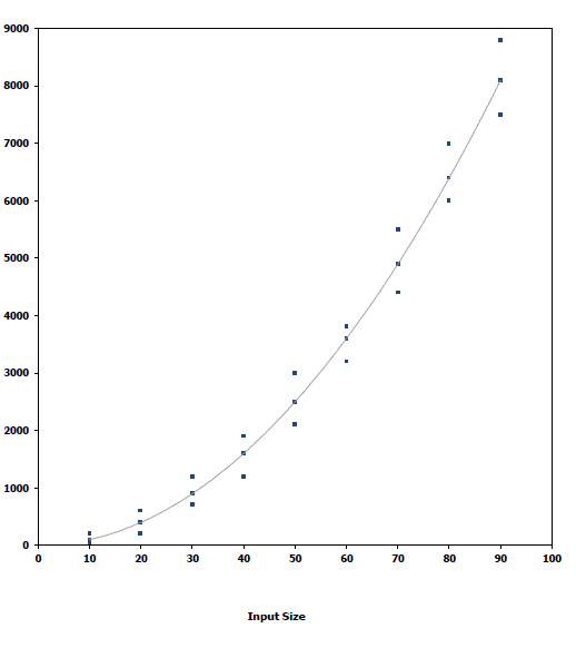
• It is necessary to implement the algorithm, which may be difficult
• Results may not be indicative of the running time on other inputs not included in the experiment.
• In order to compare two algorithms, the same hardware and software environments must be used

Theoretical Analysis

• Uses a high-level description of the algorithm instead of an implementation
• Characterizes running time as a function of the input size, n.
• Takes into account all possible inputs
• Allows us to evaluate the speed of an algorithm independent of the hardware/software environment

Simple Example

// Input: int A[N], array of N integers // Output: Sum of all numbers in array A int Sum(int A[], int N){
int s=0;
for (int i=0; i< N; i++)
    s = s + A[i];
return s; }

Simple Example: Growth of 5n+3

Estimated running time for different values of N: N = 10=> 53 steps N = 100=> 503 steps N = 1,000=> 5003 steps N = 1,000,000=> 5,000,003 steps As N grows, the number of steps grow in linear proportion to N for this function “Sum”

What Dominates in Previous Example?

What about the +3 and 5 in 5N+3?

• As N gets large, the +3 becomes insignificant
• 5 is inaccurate, as different operations require varying amounts of time and also does not have any significant importance
• What is fundamental is that the time is linear in N.

Asymptotic Complexity

• The 5N+3 time bound is said to "grow asymptotically" like N
• This gives us an approximation of the complexity of the algorithm
• Ignores lots of (machine dependent) details, concentrate on the bigger picture

Coding example 1

for ( i=0 ; i<n ; i++ ) 
    m += i;
f(n) = 4n+1

Coding example #2

for ( i=0 ; i<n ; i++ ) 
    for( j=0 ; j<n ; j++ )
	    sum[i] += entry[i][j]; f(n) = 𝟔𝒏𝟐 + 𝟑𝒏 + 𝟏

What is Rate of Growth?

• The rate at which the running time increases as a function of input is called rate of growth.
• Let us assume that you go to a shop to buy a car and a bicycle. If your friend sees you there and asks what you are buying, then in general you say buying a car. This is because the cost of the car is high compared to the cost of the bicycle (approximating the cost of the bicycle to the cost of the car).

Total cost = cost of car + cost of bicycle Total cost ≈ cost of car (approximation)

• For the above-mentioned example, we can represent the cost of the car and the cost of the bicycle in terms of function, and for a given function ignore the low order terms that are relatively insignificant (for large value of input size, n).

• As an example, in the case below, n4, 2n2, 100n and 500 are the individual costs of some function and approximate to n4 since n4 is the highest rate of growth. n4 + n2 +100n + 500 ≈ n4

  
  

Commonly Used Rates of Growth

Types of Analysis

To analyze the given algorithm, we need to know with which inputs the algorithm takes less time (performing well) and with which inputs the algorithm takes a long time. We have already seen that an algorithm can be represented in the form of an expression. That means we represent the algorithm with multiple expressions: one for the case where it takes less time and another for the case where it takes more time. In general, the first case is called the best case and the second case is called the worst case for the algorithm. To analyze an algorithm we need some kind of syntax, and that forms the base for asymptotic analysis/notation

There are three types of analysis:

• Worst case
  • Defines the input for which the algorithm takes a long time (slowest time to complete).
  • Input is the one for which the algorithm runs the slowest. • Best case
  • Defines the input for which the algorithm takes the least time (fastest time to complete).
  • Input is the one for which the algorithm runs the fastest. • Average case
  • Provides a prediction about the running time of the algorithm.
  • Run the algorithm many times, using many different inputs that come from some distribution that generates these inputs, compute the total running time (by adding the individual times), and divide by the number of trials.
  • Assumes that the input is random.

Asymptotic Notation

• Having the expressions for the best, average and worst cases, for all three cases we need to identify the upper and lower bounds.
• To represent these upper and lower bounds, we need some kind of syntax, and that is the subject of the following discussion.
• Let us assume that the given algorithm is represented in the form of function f(n).

Big-O Notation [Upper Bounding Function]

• This notation gives the tight upper bound of the given function.
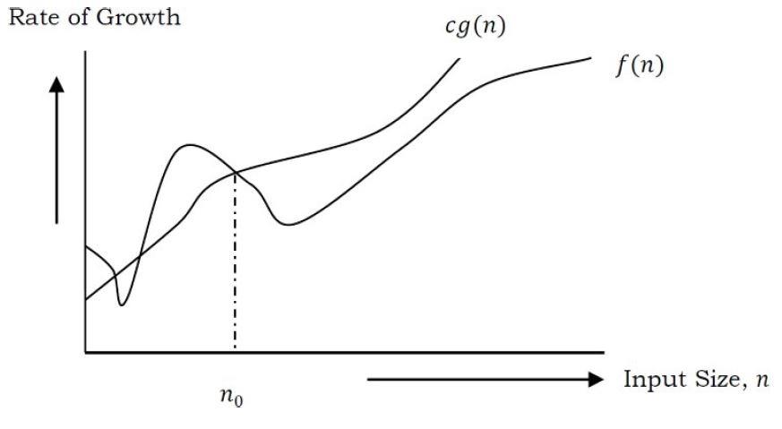
• Generally, it is represented as f(n) = O(g(n)). That means, at larger values of n, the upper bound of f(n) is g(n).
• For example, if f(n) = 𝑛4 + 100𝑛2 + 10𝑛 + 50 is the given algorithm, then 𝑛4 is g(n). That means g(n) gives the maximum rate of growth for f(n) at larger values of n.

Let us see the O–notation with a little more detail.

Definition: O–notation defined as O(g(n)) = {f(n): there exist positive constants c and 𝑛0 such that 0 ≤

f(n) ≤ cg(n) for all n > 𝑛0}. g(n) is an asymptotic tight upper bound for f(n).

• Our objective is to give the smallest rate of growth g(n) which is greater than or equal to the given algorithms’ rate of growth /(n).
• Generally we discard lower values of n. That means the rate of growth at lower values of n is not important.
• In the figure, 𝑛0 is the point from which we need to consider the rate of growth for a given algorithm. Below 𝑛0, the rate of growth could be different. 𝑛0 is called threshold for the given function

Big-O Visualization

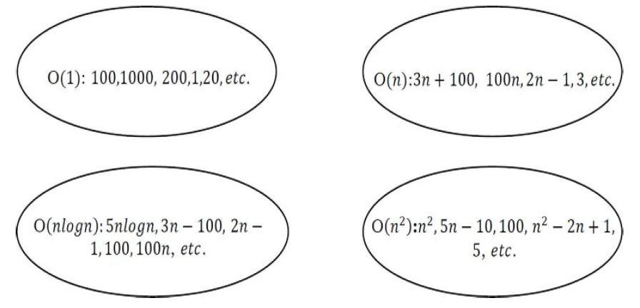
O(g(n)) is the set of functions with smaller or the same order of growth as g(n). For example; O(𝑛2) includes O(1), O(n), O(nlogn), etc. Note: Analyze the algorithms at larger values of n only. What this means is, below 𝑛0 we do not care about the rate of growth.

Example for linear function

• When we say that the function 4n+1 is Big O(n), we are saying that the asymptotic behavior of a linear function is equal to or greater than its own.
• This means that the 4n+1 function will never grow to the point where it surpasses linear behavior.
• Thus, Big O(n) presents itself as an upper limit, and we know that the function will never exhibit growth behavior that exceeds this upper limit.
• https://algol.dev/en/big-o-notation/
• Example: for function 4n+1, there is another function of linear behavior that limits it superiorly. Note in the graph below that, for values of n>1, the function 4n+1 is surpassed by another function of class n.

Similarly, it is also correct to say that 4n+1 is Big O(n2), because the 4n+1 function will never grow to the point where it exceeds quadratic behavior. Thus, O(n2) also presents itself as an upper asymptotic limit:

Now it would be wrong to say that 4n+1 is Big O(1), because the 4n+1 function will always grow to the point where it surpasses constant behavior. Thus, Big O(1) is not presented as an upper asymptotic limit:

Summing up:

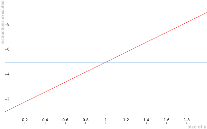
4n+1 is Big O(n2), as it can be overcome (superiorly limited) by a quadratic function. 4n+1 is Big O(n), as it can be overcome (superiorly limited) by a linear function. 4n+1 is not Big O(1), as it cannot be surpassed (superiorly limited) by a constant function.

Example for quadratic function

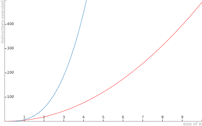
• When we say that the function 5n2-n+1 is Big O(n2), we are saying that the asymptotic behavior of a quadratic function is equal to or greater than its own.
• This means that the function 5n2-n+1 will never grow to the point where it exceeds quadratic behavior.
• Thus, O(n2) is presented as an upper limit and we know that the function will never exhibit growth behavior that exceeds this upper limit.

Example: For the 5n2-n+1 function, there is another quadratic behavior function that limits it superiorly. See below:

Similarly, it is also correct to say that 5n -n+1 is Big O(n^2), because the function 5n -n+1 will never grow to the point where it exceeds cubic behavior. Thus, O(n3) also presents itself as an upper asymptotic limit:

Now it would be wrong to say that 5n2-n+1 is Big O(n), because the function 5n2-n+1 will always grow to the point where it surpasses linear behavior. Thus, O(n) does not present itself as an upper asymptotic limit:

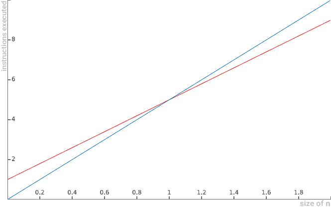
First example of mathematical use of Big O notation

• Let us try to demonstrate by definition that 4n+1=O(n) (reads “It’s Big O of n”).
• By definition, all we have to do is demonstrate that there is a positive constant c and a positive initial value n0 so that for all values of n greater than or equal to n0, 4n+1 is always less than or equal to c multiplied by n.
• In summary: we need to prove that 4n+1 ≤ c.n, for a positive c constant and a positive initial n0 value.
• To do so, the first decision we need to make is to choose a value for the constant c. In this case, let’s consider c equal to the value 5. Note below a table showing the inequality results for c=5 and for some values of n:

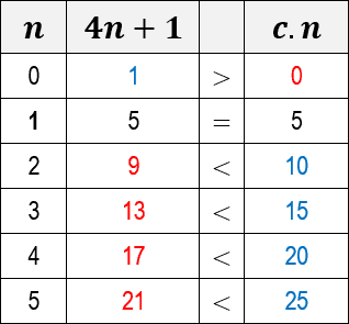
Note that for n equal to 0 (zero) the function of algorithm 4n+1 is greater than c.n. But when n equals 1, the values of c.n begin to outperform the 4n+1 algorithm. When we plot a graph for both functions, we see more clearly this exact moment of overrun of the c.n function:

• This means that O(n) represents an upper asymptotic limit for the 4n+1 function. For from a given value n, c.n surpasses the function.
• However, what really matters for algorithm analysis is that we can demonstrate our goal, namely that there is a constant c=5 and an n0=1, such that 4n+1 ≤ c.n for all n values greater than or equal to n0.
• Thus, it is proved that, in fact, 4n+1=O(n) (is Big O of n).

Second example of the mathematical use of Big O notation

• Let us try to demonstrate by definition that 5n2-n+1=O(n2) (reads “It’s Big O from n squared”).

• By definition, all we have to do is demonstrate that there is a positive constant c and a positive initial value n0 so that for all n values greater than or equal to n0​, 5n2-n+1 is always less than or 2 equal to c multiplied by n .

• In summary, we need to prove that 5n2-n+1 ≤ c.n2, for a constant c and an initial n0 value.

• Again, we need to choose a value for the constant c. In this case, we will also consider c equal to the value 5.

• Note below a table showing the inequality results for c=5 and for some values of n:

  
  

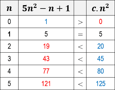
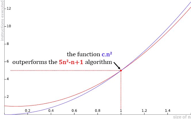
Note that for n equal to 0 (zero) the algorithm function 5n -n+1 is greater than c.n . But when n equals 1 the values of c.n2 begin to outperform the algorithm 5n2-n+1. When we plot a graph for both functions, we see more clearly this exact moment of overrun of the c.n2 function:

• This means that O(n2) represents an upper asymptotic limit for the 5n2-n+1 function.

• For from a given value n, c.n2 surpasses the function. However, what really matters for algorithm analysis is that we can demonstrate our goal, that there is a constant c=5 and n0=1, such that 5n2-n+1 ≤ c.n2 for all n values greater than or equal to n0.

• Thus, it is proved that, in fact, 5n2-n+1=O(n2) (is Big O from n squared).

  
  

Third example: a failed attempt

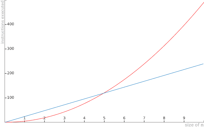
• Let’s try to demonstrate by definition that 2n2-n=O(n).
• By definition, all we have to do is demonstrate that there is a positive constant c and an initial value n0 so that for all values greater than n0, 2n2-n is always less than or equal to c multiplied by n.
• In summary, we need to prove that 2n2-n≤c.n, for a constant c and an initial n0 value
• At first glance, it is clear that 2n2-n has quadratic behavior and c.n has linear behavior.
• So we are tempted to claim that this demonstration is false, since a linear function (c.n) cannot represent an upper asymptotic limit for a quadratic function (2n2-n).
• But let’s take a closer look to see why this is impossible.

Let’s perform some algebraic transformations in order to isolate the constant c in inequality and understand its possible values:

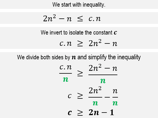
• The resulting inequality already shows us that it is impossible for any constant c to make the expression valid for large values of n (n→∞), because no matter how large the value of c is, the value of n will always exceed it.
• Below are some graphs illustrating some scenarios of c.n being overcome by the 2n2-n quadratic function:

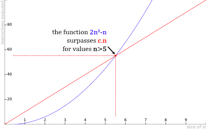
Below are some graphs illustrating some scenarios of c.n being overcome by the 2n2-n quadratic function:

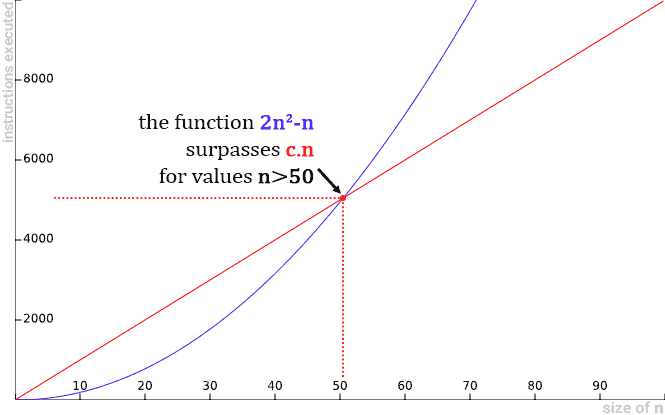
• That is, no matter how large the constant c. The 2n2-n function will always outperform the c.n.
• Therefore, we cannot demonstrate our goal. There is no constant c and n0, such that 2n2-n ≤ c.n for all n values greater than or equal to n0. Thus, it is proved that, in fact, 2n2-n≠O(n) (reads “it’s not Big O of n”).

Reference

1. Chapter 3 (Introduction to Algorithms, second edition, T.H.Cormen, C.E.Leiserson, R.L.Rivest,and C.Stein,PHI Pvt. Ltd./ Pearson Education)
2. Chapter 1 (Data Structures and Algorithms Made Easy: Data Structures and Algorithmic Puzzles, Narasimha Karumanchi)
3. https://algol.dev/en/big-o-notation/

TODO:

5. Arrays
6. Stacks
7. Stack Applications
8. Recursion
9. Queues
10. Searching
11. Sorting
12. Quick sort
13. Heap sort
14. Trees

To be continued...